Here are Madeline’s Exam 3 notes, organized to help you focus on the ideas most likely to appear on the test.
📄 PDF version:
Download MATH 116 – EXAM 3 (Madeline’s Review Sheet)
Exam 3 Review Problems
116 Exam3 Review (Fall 2025)-1
Last years exam 2024 116 Exam3 Review (Fall 2024)-1
Use them for review and practice:
- Work through problems
- Check each topic
- Let yourself make mistakes now, not on the exam
If you get stuck or something does not quite click, message your TAs. Hope this helps, and enjoy Thanksgiving break.
1. Exponential Functions
An exponential function has the form
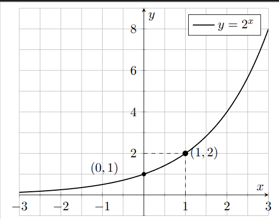
- If \(b > 1\) then we’ve got exponential growth
- If \(0 < b < 1\): exponential decay
Key graph features:
- Horizontal asymptote: \(y = 0\). Basic exponential functions \(b^x\) are always positive.
- Graph never touches the \(x\)-axis.
- Always passes through \((0,1)\) because \(b^0 = 1\).
Transformations:
- \(f(x) = a \, b^x\)
- \(|a|>1\): vertical stretch
- \(0<|a|<1\): vertical shrink
- \(a<0\): reflection across the \(x\)-axis.
- \(f(x) = b^{x-h}\): horizontal shift right by \(h\).
- \(f(x) = b^x + k\): vertical shift up by \(k\).
- Asymptote becomes \(y = k\).
2. Logarithms
Logarithms are just exponents in disguise:
\[ \log_b(x) = y \quad \Longleftrightarrow \quad b^y = x. \]Special case: the natural log:
\[ \ln(x) = \log_e(x). \]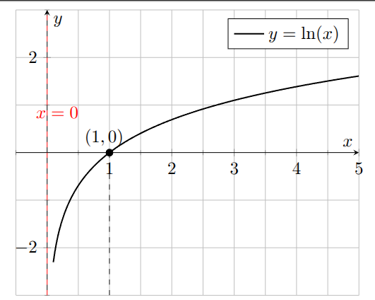
Log rules you must know:
- Product: \[ \ln(ab) = \ln(a) + \ln(b) \]
- Quotient: \[ \ln\!\left(\frac{a}{b}\right) = \ln(a) - \ln(b) \]
- Power: \[ \ln(a^p) = p \ln(a) \]
These are your “log superpowers” for simplifying expressions and solving equations.
Graph features of \(y = \ln x\):
- Vertical asymptote: \(x = 0\).
- Domain: \(x > 0\).
- Passes through \((1, 0)\).
3. Solving Exponential and Log Equations
Typical strategy:
- Isolate the exponential or logarithm.
- If it’s exponential, use logs. If it’s logarithmic, change to exponential form.
- If solving for time \(t\), you’ll almost always end up using \(\ln\).
- Use log rules to bring exponents down.
- Solve for the variable like a normal algebra equation.
Important tips:
If you can rewrite both sides with the same base, set exponents equal.
$$b^{\text{something}} = b^{\text{something\_else}}.$$Then,
$$ \text{something} = \text{something else} $$If the bases do not match nicely, use \(\ln\) (or \(\log\)).
4. Compound Interest
Money stuff! The standard formula (compounded a finite number of times per year):
\[ A = P \left(1 + \frac{r}{n}\right)^{nt}, \]where
- \(P\): principal (starting amount)
- \(r\): annual interest rate (as a decimal)
- \(n\): number of compounding periods per year
- \(t\): time in years
- \(A\): final amount (the “after” picture)
Continuously compounded interest:
\[ A = P e^{rt}. \]If you see the word “continuously,” your reflex should be: “That’s an \(e^{rt}\) situation.”
5. Effective Annual Rate
The effective annual rate says: “If I had just one compounding per year, what single rate would give the same result?”
If interest is compounded \(n\) times per year:
\[ r_{\text{eff}} = \left(1 + \frac{r}{n}\right)^n - 1 \]If interest is compounded continuously:
\[ r_{\text{eff}} = e^r - 1 \]
Interpretation:
Bigger \(r_{\text{eff}}\) = better investment (for you). Worse for your credit card bill.
6. Derivatives of Exponential and Log Functions
Core derivative facts to memorize:
- \[ \frac{d}{dx}\big[e^x\big] = e^x \]
- \[ \frac{d}{dx}\big[a^x\big] = a^x \ln(a), \quad a>0,\ a\neq1 \]
- \[ \frac{d}{dx}\big[\ln(x)\big] = \frac{1}{x}, \quad x>0 \]
Chain rule forms:
- \[ \frac{d}{dx}\big[e^{g(x)}\big] = g'(x)\, e^{g(x)} \]
- \[ \frac{d}{dx}\big[\ln(g(x))\big] = \frac{g'(x)}{g(x)} \]
And just like on Exam 2, be ready to combine:
- Product rule
- Quotient rule
- Chain rule
7. Antiderivatives (Indefinite Integrals)
Antiderivatives are “derivatives in reverse.” General formulas:
- For \(n \neq -1\): \[ \int x^n \, dx = \frac{x^{n+1}}{n+1} + C \]
- Exponential base \(e\): \[ \int e^x \, dx = e^x + C \]
- Exponential base \(a\): \[ \int a^x \, dx = \frac{a^x}{\ln(a)} + C, \quad a>0,\ a\neq1 \]
- Log-type integrand: \[ \int \frac{1}{x} \, dx = \ln|x| + C \]
Pro-tip:
Take the derivative of your answer to check:
If yes → happy dance. If no → find where you made a mistake.
8. Approximating Area (Riemann Sums)
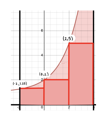
Idea: Approximate area under the curve using rectangles.
On interval \([a,b]\) with \(n\) rectangles:
\[ \Delta x = \frac{b - a}{n} \]Then area is approximately:
\[ \text{Area} = \text{(height)} \cdot \text{width} \]The height depends on which method:
Left endpoints:
\[ L_n = \sum_{i=1}^{n} f(x_{i-1})\,\Delta x \]Right endpoints:
\[ R_n = \sum_{i=1}^{n} f(x_i)\,\Delta x \]Midpoints:
\[ M_n = \sum_{i=1}^{n} f\!\left(\frac{x_{i-1}+x_i}{2}\right)\,\Delta x \]
9. Fundamental Theorem of Calculus (FTC)
This is the bridge between derivatives and integrals.
FTC Part 2
If \(F\) is an antiderivative of \(f\), then
\[ \int_a^b f(x)\,dx = F(b) - F(a). \]So to compute a definite integral:
- Find an antiderivative \(F(x)\).
- Plug in the upper limit and lower limit: \[ F(b) - F(a). \]
Net Change Formula
If \(F\) is some “quantity” whose rate of change is \(F'(x) = f(x)\), then
\[ F(b) = F(a) + \int_a^b f(x)\,dx. \]Interpretation:
New amount = old amount + total accumulated change.
This shows up in “total change” problems: total distance traveled, total money earned, total water pumped, etc.